Determination of Caffeine in Coffee Using High Performance Thin Layer Chromatography
Read more about
Introduction
High Performance Thin Layer Chromatography (HPTLC) is a very useful analytical technique and requires low sample preparation, here illustrated through the analysis of caffeine in coffee. Only extraction and filtration, through a 0.45 μm PTFE syringe filter, is needed for boiled coffee samples prior analysis. The HPTLC plate was pre-conditioned with the mobile phase, and a TLC-scanner was a used for the quantitation after the chromatographic separation was completed.
Results and Discussion
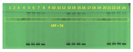
Caffeine was detected under UV light at 254 nm, hRf = 56, (Figure 1). A four-level calibration curve was constructed and used for quantitation purposes, (Figure 2). Each sample was analyzed in triplicate performed in parallel, a benefit with planar chromatography over both GC and HPLC.

Figure 1.Developed HPTLC plate at 254 nm, chromatographic data shown in the table above.

Figure 2.Calibration graph following the polynomial regression mode (r = 0.9970).
To continue reading please sign in or create an account.
Don't Have An Account?